Support Vector Machine in R: A Step-by-Step Tutorial

Some algorithms fall out of fashion without losing their usefulness. The support vector machine is one of them. On small to medium datasets with clear class separation, it still competes with far heavier methods — and it trains in seconds.

Building a support vector machine in R is refreshingly direct. The e1071 package wraps the battle-tested libsvm library, giving you classification, regression and automatic hyperparameter tuning in a handful of lines.

This tutorial walks through the concept, the code pattern, the parameters that actually matter, and the mistakes that quietly wreck results.

What Is a Support Vector Machine?

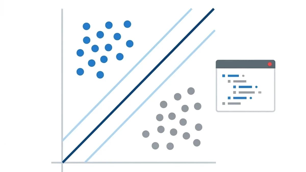
A support vector machine is a supervised learning algorithm that finds the decision boundary separating classes with the widest possible margin. Instead of merely drawing any dividing line, it draws the line that stays furthest from the nearest points of each class.

Those nearest points are the support vectors, and they alone define the boundary. This is why SVMs are memory-efficient and relatively robust on smaller datasets — most training points have no influence once the margin is set.

When classes are not linearly separable, the kernel trick maps data into a higher-dimensional space where a linear split becomes possible, without ever computing those coordinates explicitly. The radial basis function kernel is the practical default for most real data.

Who Uses SVMs in R?

R remains the environment of choice wherever statistical rigour and reporting matter more than production scale.

• Academic researchers in bioinformatics, where gene expression datasets have many features and few samples — SVM's sweet spot.
• Risk analysts building credit default and fraud classifiers on structured historical data.
• Marketing analysts scoring lead conversion likelihood from CRM and campaign attributes.
• Medical and clinical researchers classifying diagnostic outcomes from measurement panels.
• Students and data science learners because R's syntax makes the mechanics visible rather than hidden.

Key Concepts You Must Understand First

The Kernel Choice

Linear kernels work when the relationship is roughly additive and the feature count is high. Radial kernels handle curved boundaries and are the sensible starting point otherwise. Polynomial kernels exist but rarely outperform radial in practice.

Cost (C) and Gamma

Cost controls the penalty for misclassifying training points — high C means a tighter fit and more overfitting risk. Gamma controls how far a single point's influence reaches in the radial kernel. These two parameters dominate performance, and tuning them together is essential.

Feature Scaling

SVMs are distance-based, so a variable measured in thousands will dominate one measured in decimals. The svm() function scales by default, which is helpful — but if you disable it, standardise manually or expect poor results.

Class Imbalance

With 95% negatives, an SVM can score 95% accuracy while never predicting the positive class. Use class weights, resampling, and evaluate with precision, recall and F1 rather than accuracy.

How to Build a Support Vector Machine in R

The workflow below is the standard pattern. Keep the steps in order — particularly the train/test split before any tuning.

1. Install and load the package. Run install.packages("e1071") then library(e1071). Add caret for convenient splitting and confusion matrices.
2. Prepare your data. Ensure the target variable is a factor for classification; a numeric target triggers regression mode instead.
3. Split into training and test sets. A 70/30 or 80/20 split is conventional. Set a seed so results are reproducible.
4. Fit a baseline model. Call svm(target ~ ., data = train, kernel = "radial") and inspect the summary for support vector counts.
5. Tune the hyperparameters. Use tune.svm() over a grid of cost and gamma values — it runs cross-validation and returns the best combination.
6. Retrain with the best parameters and predict on the held-out test set using predict().
7. Evaluate properly. Build a confusion matrix and report precision, recall and F1 per class, not just overall accuracy.

Benefits of Using SVMs

SVMs remain a strong default for a specific and common situation: modest data, many features, clear decision task.

• Strong performance in high-dimensional space, even when features outnumber observations.
• Effective margin-based regularisation that resists overfitting when C is tuned sensibly.
• Flexible boundaries via kernels without redesigning the model architecture.
• Fast training on small datasets, often seconds versus minutes for ensemble methods.
• Deterministic results, which matters for reproducible research and audit trails.

Potential Challenges

SVMs have real limits, and pretending otherwise leads to frustration on larger projects.

• Poor scaling to large datasets. Training time grows roughly quadratically, so tens of thousands of rows becomes slow.
• Limited interpretability. A radial-kernel boundary cannot be explained as neatly as regression coefficients.
• No native probability output. You must set probability = TRUE and accept the extra fitting cost.
• Sensitivity to hyperparameters. Untuned C and gamma can swing accuracy by twenty points or more.

Best Practices and Tips

Most SVM disappointments trace back to one of these four omissions.

• Always tune cost and gamma together with cross-validation; tuning one at a time misses the interaction.
• Verify scaling is applied, especially when mixing units like age, income and ratios.
• Compare against a random forest baseline. If the ensemble wins clearly, use it — loyalty to an algorithm is not a strategy.
• Keep the test set untouched until final evaluation. Tuning on test data inflates every number you report.

Real-World Example

A credit union wanted to flag loan applications likely to default. They had 3,400 historical applications with 22 features: income, debt ratio, employment length, prior delinquencies and similar fields. The default rate was 14%, so imbalance mattered.

An initial radial SVM with default settings achieved 86% accuracy but recall of only 0.31 on defaults — it was mostly predicting the majority class. After running tune.svm() across cost values from 0.1 to 100 and gamma from 0.001 to 1, and adding class weights inversely proportional to frequency, recall rose to 0.68 while precision held near 0.52. That trade-off was acceptable to the risk team, since a flagged application only triggered manual review rather than automatic rejection. The scored output was piped into their internal review dashboard, built as part of a wider custom web application project so underwriters saw the risk score alongside each file.

Why It Matters

Knowing when a lighter, older method suffices is a genuine professional skill. Reaching for deep learning on 3,000 rows wastes time and produces worse, less explainable results than a well-tuned SVM.

Equally important is what happens after the model works. A classifier only creates value once its predictions reach the people making decisions, which usually means an API and interface delivered through solid back-end development rather than a script on an analyst's laptop.

Frequently Asked Questions

Which R package is best for SVM?

The e1071 package is the standard choice and wraps libsvm directly. kernlab offers more kernel options, and caret or tidymodels provide unified tuning workflows around both.

Should I use a linear or radial kernel?

Start with radial for most tabular data. Choose linear when you have very many features relative to observations, such as text vectors, where linear often performs equally well and trains far faster.

How large can my dataset be?

SVMs are comfortable up to roughly 10,000–50,000 rows depending on features and hardware. Beyond that, gradient boosting or a linear SVM variant will train far faster with comparable accuracy.

Can an SVM do regression?

Yes. If the target variable is numeric rather than a factor, svm() automatically performs support vector regression, controlled by an additional epsilon parameter.

Conclusion

A support vector machine in R is a fast, reliable tool for the many problems that do not need a neural network. Scale your features, tune cost and gamma with cross-validation, evaluate on untouched test data, and compare honestly against a simpler baseline.

Once your model performs, the next step is deployment. Consider specialist AI and machine learning services to move it from an R script into a system your team can actually use daily.